Graph
Overview
This document provides a detailed comparison between different graph representations in Java, including Adjacency Matrix and Adjacency List. It covers their structures, operations, performance characteristics, visualizations, and practical applications. We’ll also explore a LeetCode example (Clone Graph) that combines graph and hash map usage.
Basic Definitions
What is a Graph?
A graph is a data structure consisting of a set of vertices (nodes) and a set of edges connecting pairs of vertices. Graphs can be:
- Directed (edges have direction)
- Undirected (edges have no direction)
- Weighted (edges have weights)
- Unweighted (edges have no weights)
Types of Graphs
- Undirected Unweighted Graph: Social networks, friend relationships
- Directed Weighted Graph: Road networks, flight routes
Visual Representation
Below is a simple undirected graph with 4 nodes and 5 edges:
   0
  / \
 1---2
  \ /
   3
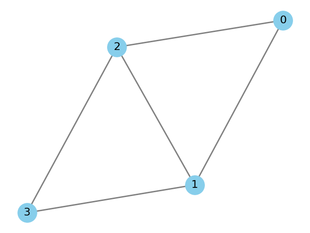 Figure: A simple undirected graph with 4 nodes and 5 edges.
In the following sections, we will use this graph as an example to illustrate both the adjacency matrix and adjacency list representations.
Adjacency Matrix Representation
  0 1 2 3
0 0 1 1 0
1 1 0 1 1
2 1 1 0 1
3 0 1 1 0
Figure: Adjacency matrix representation of the above graph.
The adjacency matrix is a 2D array where the entry at row i and column j is 1 if there is an edge between node i and node j, and 0 otherwise. This representation is simple and allows for fast edge lookups (O(1)), but it uses O(V²) space, making it inefficient for large, sparse graphs. It is best suited for dense graphs where most pairs of nodes are connected.
Adjacency List Representation
0: 1, 2
1: 0, 2, 3
2: 0, 1, 3
3: 1, 2
Figure: Adjacency list representation of the above graph.
The adjacency list uses an array (or list) of lists, where each index represents a node and stores a list of its neighbors. This approach is memory-efficient for sparse graphs (O(V+E) space) and is the most common representation in practice. However, checking if an edge exists between two nodes may take O(degree) time, where degree is the number of neighbors of a node.
Mathematical Perspective: Laplacian Matrix and Eigenvalues
For a graph with adjacency matrix \(A\) and degree matrix \(D\) (where \(D_{ii}\) is the degree of node \(i\)), the Laplacian matrix \(L\) is defined as:
\[L = D - A\]The eigenvalues of \(L\) are real and non-negative. The second smallest eigenvalue, usually denoted as \(\lambda_2\), is called the algebraic connectivity of the graph.
- \(\lambda_2 > 0\) if and only if the graph is connected.
- The larger \(\lambda_2\), the more robustly connected the graph is.
- \(\lambda_2\) is widely used in spectral graph theory, network robustness, and consensus algorithms.
Example: For the above graph, you can compute $L$ and its eigenvalues to analyze its connectivity properties.
Visualizing $\lambda_2$ in Different Graphs
Below is a comparison of three graphs with different connectivity properties. The value of \(\lambda_2\) is shown in each subfigure title:
 Figure: Left: Disconnected graph (\(\lambda_2 = 0\)). Middle: Connected but sparse graph (small \(\lambda_2\)). Right: Connected and dense graph (large \(\lambda_2\)).
- Left: The graph is disconnected, so \(\lambda_2 = 0\).
- Middle: The graph is globally connected but has few edges, so $\lambda_2$ is positive but small, indicating weak connectivity.
- Right: The graph is globally connected and has many edges, so $\lambda_2$ is much larger, indicating strong connectivity and robustness.
This demonstrates how $\lambda_2$ quantitatively reflects the overall connectivity of a graph.
Structural Comparison
| Aspect | Adjacency Matrix | Adjacency List |
|---|---|---|
| Space Complexity | O(V^2) | O(V + E) |
| Edge Lookup | O(1) | O(degree) |
| Add Edge | O(1) | O(1) |
| Remove Edge | O(1) | O(degree) |
| Iterate Neighbors | O(V) | O(degree) |
| Best For | Dense graphs | Sparse graphs |
- V: number of vertices
- E: number of edges
Implementation in Java
Adjacency Matrix (Undirected Graph)
class GraphMatrix {
    private int V;
    private int[][] matrix;

    public GraphMatrix(int V) {
        this.V = V;
        matrix = new int[V][V];
    }

    public void addEdge(int u, int v) {
        matrix[u][v] = 1;
        matrix[v][u] = 1; // undirected
    }

    public void removeEdge(int u, int v) {
        matrix[u][v] = 0;
        matrix[v][u] = 0;
    }

    public boolean hasEdge(int u, int v) {
        return matrix[u][v] == 1;
    }

    public void printMatrix() {
        for (int i = 0; i < V; i++) {
            for (int j = 0; j < V; j++) {
                System.out.print(matrix[i][j] + " ");
            }
            System.out.println();
        }
    }
}
Adjacency List (Undirected Graph)
import java.util.*;

class GraphList {
    private int V;
    private List<List<Integer>> adj;

    public GraphList(int V) {
        this.V = V;
        adj = new ArrayList<>();
        for (int i = 0; i < V; i++) {
            adj.add(new ArrayList<>());
        }
    }

    public void addEdge(int u, int v) {
        adj.get(u).add(v);
        adj.get(v).add(u); // undirected
    }

    public void removeEdge(int u, int v) {
        adj.get(u).remove((Integer)v);
        adj.get(v).remove((Integer)u);
    }

    public boolean hasEdge(int u, int v) {
        return adj.get(u).contains(v);
    }

    public void printList() {
        for (int i = 0; i < V; i++) {
            System.out.print(i + ": ");
            for (int vtx : adj.get(i)) {
                System.out.print(vtx + " ");
            }
            System.out.println();
        }
    }
}
Common Operations
Add Node / Edge
- Adjacency Matrix: Add row/column (resize array), set matrix[u][v] = 1
- Adjacency List: Add new list, add to neighbor lists
Remove Node / Edge
- Adjacency Matrix: Set matrix[u][v] = 0
- Adjacency List: Remove from neighbor lists
Search / Traversal
- BFS (Breadth-First Search)
- DFS (Depth-First Search)
BFS Example (Adjacency List)
public void bfs(int start) {
    boolean[] visited = new boolean[V];
    Queue<Integer> queue = new LinkedList<>();
    visited[start] = true;
    queue.offer(start);
    while (!queue.isEmpty()) {
        int u = queue.poll();
        System.out.print(u + " ");
        for (int v : adj.get(u)) {
            if (!visited[v]) {
                visited[v] = true;
                queue.offer(v);
            }
        }
    }
}
DFS Example (Adjacency List)
public void dfs(int u, boolean[] visited) {
    visited[u] = true;
    System.out.print(u + " ");
    for (int v : adj.get(u)) {
        if (!visited[v]) {
            dfs(v, visited);
        }
    }
}
Performance Analysis
| Operation | Adjacency Matrix | Adjacency List |
|---|---|---|
| Add Edge | O(1) | O(1) |
| Remove Edge | O(1) | O(degree) |
| Check Edge | O(1) | O(degree) |
| Enumerate Neigh. | O(V) | O(degree) |
| Space | O(V^2) | O(V+E) |
- Adjacency Matrix is better for dense graphs (many edges)
- Adjacency List is better for sparse graphs (few edges)
Applications
- Social Networks: Users and friendships (undirected, sparse)
- Maps/Navigation: Cities and roads (directed, weighted)
- Web Links: Pages and hyperlinks (directed)
- Scheduling: Tasks and dependencies (DAG)
- Network Routing: Routers and connections
LeetCode Example: 133. Clone Graph (with HashMap)
Problem
Given a reference of a node in a connected undirected graph, return a deep copy (clone) of the graph. Use a hash map to avoid revisiting nodes.
Java Solution (DFS + HashMap)
class Node {
    public int val;
    public List<Node> neighbors;
    public Node() {
        val = 0;
        neighbors = new ArrayList<Node>();
    }
    public Node(int _val) {
        val = _val;
        neighbors = new ArrayList<Node>();
    }
    public Node(int _val, ArrayList<Node> _neighbors) {
        val = _val;
        neighbors = _neighbors;
    }
}

class Solution {
    private Map<Node, Node> visited = new HashMap<>();

    public Node cloneGraph(Node node) {
        if (node == null) return null;
        if (visited.containsKey(node)) {
            return visited.get(node);
        }
        Node clone = new Node(node.val);
        visited.put(node, clone);
        for (Node neighbor : node.neighbors) {
            clone.neighbors.add(cloneGraph(neighbor));
        }
        return clone;
    }
}
Explanation:
- Use a HashMap<Node, Node> to map original nodes to their clones.
- Prevents infinite loops and duplicate nodes.
- Works for any connected undirected graph.
More LeetCode Graph Problems
-
- Course Schedule (Topological Sort)
-
- Number of Islands (DFS/BFS)
-
- Is Graph Bipartite?
Summary Table
| Representation | Space | Edge Lookup | Add Edge | Remove Edge | Iterate Neighbors | Best For |
|---|---|---|---|---|---|---|
| Adjacency Matrix | O(V^2) | O(1) | O(1) | O(1) | O(V) | Dense Graphs |
| Adjacency List | O(V + E) | O(degree) | O(1) | O(degree) | O(degree) | Sparse Graphs |
| Edge List | O(E) | O(E) | O(1) | O(E) | O(E) | Simple Graphs |
Key Takeaways
- Adjacency Matrix is simple and fast for dense graphs, but wastes space for sparse graphs.
- Adjacency List is memory-efficient for sparse graphs and is the most common representation.
- Edge List is useful for algorithms that process all edges (e.g., Kruskal’s MST).
- HashMap is often used in graph algorithms to track visited nodes or mappings (see LeetCode 133).
- Choose the representation based on the graph’s density and the operations you need to optimize.