Control Barrier Function

Finished

Consider a control-affine dynamical system defined as:

\[\dot{\mathbf{x}} = f(\mathbf{x}) + g(\mathbf{x})u\]

where \(\mathbf{x}\in\mathcal{X}\sub\mathbb{R}^{d}\), \(\mathbf{u}\in\mathcal{U}\sub\mathbb{R}^{q}\) denotes the control input. \(f:\mathbb{R}^{d} \mapsto \mathbb{R}^{d}\) and \(g\!:\!\mathbb{R}^{d}\!\mapsto\!\mathbb{R}^{d\times q}\) are locally Lipschitz continuous.

Theorem Control Barrier Function

(Safety) Considering the safety radius \(R_\mathrm{s}\in\mathbb{R}\), if we want to ensure that the robots \(i\) and \(j\) are not collide with each other, we can define such set as:

\[h^\mathrm{s}_{i,j}(\mathbf{x}) = ||\mathbf{x}_i -\mathbf{x}_j||^2 -R_\mathrm{s}^2, \forall i>j\\ \mathcal{H}^\mathrm{s}_{i,j} = \{\mathbf{x} \in \mathbb{R}^{dN} | h^\mathrm{s}_{i,j}(\mathbf{x}) \geq 0 \}\]

Then, we have the following theorem:

Theorem 1 (Control Barrier Function): Given a deterministic dynamical system affine in control (i.e., \(\dot{\mathbf{x}}=F(\mathbf{x})+G(\mathbf{x})\mathbf{u}\)) and a desired set \(\mathcal{H}\) as the 0-super level set of a continuously differentiable function \(h: \mathcal{X} \mapsto \mathbb{R}\), the function $h$ is called a control barrier function, if there exists an extended class-\(\mathcal{K}\) function \(\kappa(\cdot)\) such that

\[\sup_{\mathbf{u}\in\mathcal{U}}\{\dot{h}(\mathbf{x}, \mathbf{u})\}\geq -\kappa(h(\mathbf{x}))\]

for all \(\mathbf{x}\in\mathcal{X}\) .

Question 1 why this cosntraint can enfore the forward invariance of the set \(\mathcal{H}\)?

Let’s make it formal! We can define the problem as:

Problem 1: Given the initial time step \(t = 0\) , \(h(\mathbf{x}(0))\geq0\) and \(\dot{h}(\mathbf{x})\geq-\alpha(h(\mathbf{x}))\) holds for all \(t\geq0\), then \(h(\mathbf{x}(t))\geq0\) for all \(t\geq0\).

First, let’s define an auxiliary function as:

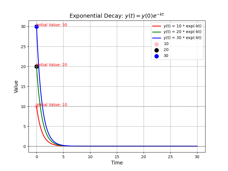
\[\frac{d}{dt}y(t) = -\alpha(y(t)), \quad y(0) = h(x(0))\]

An example for such function is that \(y(t) = e^{-\alpha t}y(0)\). This equation describes an independent system where the rate of the change of \(y(t)\) is proportional to the value of \(y(t)\) itself.

import numpy as np
import matplotlib.pyplot as plt

k = 1.0
h0 = 10
h1 = 20
h2 = 30
t = np.linspace(0, 30, 1000)


def y(t, h0, k):
    return h0 * np.exp(-k * t)

y_t = y(t, h0, k)
y_t1 = y(t, h1, k)
y_t2 = y(t, h2, k)
plt.figure(figsize=(8, 6))

plt.plot(t, y_t, 'r', label='y(t) = 10 * exp(-kt)', linewidth = 2)
plt.plot(t, y_t1, 'g', label='y(t) = 20 * exp(-kt)', linewidth = 2)
plt.plot(t, y_t2, 'b', label='y(t) = 30 * exp(-kt)', linewidth = 2)

plt.scatter(0, h0, color='pink', label='10', s=100)
plt.scatter(0, h1, color='black', label='20', s=100)
plt.scatter(0, h2, color='blue', label='30', s=100)

plt.text(0, h0 + 0.05, f'Initial Value: {h0}', color='red', fontsize=10)
plt.text(0, h1 + 0.05, f'Initial Value: {h1}', color='red', fontsize=10)
plt.text(0, h2 + 0.05, f'Initial Value: {h2}', color='red', fontsize=10)

# Plot settings
plt.title('Exponential Decay: $y(t) = y(0) e^{-kt}$', fontsize=14)
plt.xlabel('Time', fontsize=12)
plt.ylabel('Value', fontsize=12)
plt.axhline(0, color='black', linewidth=1, linestyle='--')
plt.axhline(h0, color='grey', linewidth=1, linestyle='--')
plt.axhline(0, color='grey', linewidth=1, linestyle='--')
plt.grid(True)
plt.legend()
plt.show()

See implementation for Gif

Then, we can get the following equation: Definition 1 (Class-\(\mathcal{K}\) funciton): The Class \(\mathcal{K}\) function is a function \(\alpha: \mathbb{R}_{\geq 0} \mapsto \mathbb{R}_{\geq 0}\) that is continuous, strictly increasing, and \(\alpha(0) = 0\).

Since \(\alpha\) is a class-\(\mathcal{K}\) function, we can get the \(\alpha(h)\) is monotonically increasing with \(\alpha (0) = 0\), we can intituively know that \(y(t)\) will remain non-negaitve. When the \(y(t)\rightarrow0\), the decrease rate of \(y(t)\)s, (i.e., \(\frac{d}{dt}y(t)\rightarrow 0\)) will approach to zero.

Therefore, if we can get if the change rate of \(h(\mathbf{x}(t))\) is always larger than the change rate of \(y(t)\), we can ensure that \(h(\mathbf{x}(t))\geq0\) for all \(t\geq0\). That means the decrease speed is lower than the decrease speed of \(y(t)\). With this, we can get easily conclude the conclusion.