Two Gaussian Multiplication
Working on it! ![]()
Gaussian Distribution Preliminaries
The Gaussian distribution material can be easily found in many textbooks. Here we directly define the random variable \(x\) and \(y\) as:
\[x \sim \mathcal{N}(\mu_x, \Sigma_x) \tag{1}\] \[y \sim \mathcal{N}(\mu_y, \Sigma_y) \tag{2}\]where \(\mu_x\) and \(\mu_y\) are the mean of the Gaussian distribution, and \(\Sigma_x\) and \(\Sigma_y\) are the covariance matrix of the Gaussian distribution.
Here we are interested in the distribution of the random variable \(z\), which is the multiplication of \(x\) and \(y\):
\[z =xy \tag{3}\]Question 1: What is the distribution of the random variable \(z\)?
Let’s play with the example to visualize the distribution of the random variable \(z\).
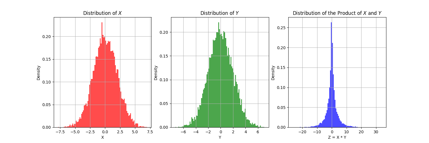
It looks like a Gaussian distribution, right? But is this true? ![]()
Let’s dig into the details! ![]()
First, we can use an relative easy way as described in this link:
The basic idea is that:
\[(x+y)^2 = x^2 + 2xy + y^2\] \[(x-y)^2 = x^2 - 2xy + y^2\]So
\[xy = \frac{1}{4}[(x+y)^2 - (x-y)^2]\] \[xy \sim \frac{\mathrm{Var}(x+y)}{4} \mathcal{Q} + \frac{\mathrm{Var}(x-y)}{4} \mathcal{R}\]where \(\mathcal{Q}\) and \(\mathcal{R}\) are central chi-square distribution. So the distribution of \(z\) is a linear combination of two central chi-square distribution.
To make it more formal, we should use the characteristic function to derive the distribution of \(z\). ![]()
Actually, we can get that:
\[f_z(z) = \frac{1}{\pi} K_0(|z|) \quad\quad |z| >0\]where \(K_0\) is the modified Bessel function of the second kind of order 0. It shows that the distribution of the random variable \(z\) is a k-form Bessel distribution. :sunglasses
Let’s visualize ![]() this process!
this process!

import numpy as np
import matplotlib.pyplot as plt
from scipy.special import kv ## Bessel function
from scipy.stats import norm

Sample = 1000
mu_x = 0
mu_y = 0
sigma_x = 1
sigma_y = 1

## Gaussian Distribution

x = np.random.normal(mu_x, sigma_x, Sample)
y = np.random.normal(mu_y, sigma_y, Sample)

## Product of two Gaussian Distribution

z = x * y

## Theoretical Distribution
def pdf_z(z):
    return (1 / (np.pi * sigma_x * sigma_y)) * kv(0, np.abs(z) / (sigma_x * sigma_y))

z_v = np.linspace(np.min(z), np.max(z), 10000)
pdf_z = pdf_z(z_v)

# Plot
plt.figure(figsize=(10, 6))
plt.hist(z, bins=200, density=True, alpha=0.6, label='Histogram of x * y')
plt.plot(z_v, pdf_z, 'r', label='Theoretical PDF $K$-from Bessel distribution')

plt.xlabel('z = x * y')
plt.ylabel('Probability Density')
plt.title('Distribution of the Product of Two Gaussian Variables')
plt.legend()
plt.grid(True)
plt.show()
Thats it! ![]() This property may be very useful in future work!
This property may be very useful in future work! ![]()